March 23 2024
Building a 10-Million Parameter LLM with 300 Lines of Python and Training It in 10 Minutes

OpenAI’s ChatGPT, Google’s Gemini, Meta’s Llama2, Mistral’s Mixtral are all examples of large languages models (LLMs). They are general-purpose machine learning models that can handle a wide variety of tasks. They seem magical, but we can build a small-scale 10-million parameter example of an LLM in around 300 lines of Python and train it in ten minutes on Google Colab for free. As we’ll see, creating and training a model is easy; achieving good performance is difficult.
The steps we’ll go through are:
- Creating a data set to train on
- Creating a machine learning model
- Training the model on the data set
- Running inference on the model
- Thinking about leaky abstractions
Throughout this post, I’ll be using machine learning terminology. See my post A Glossary for Understanding Large Language Models in AI such as OpenAI’s GPT-4, Meta’s Llama2, and Google’s Gemini for any unfamiliar terms.
Let’s get started. All the code is available at github.com/bdunagan/bdunaganGPT.
Data Set
For a small data set, I compiled a single text document with the contents of every blog post on this blog, bdunagan.com. The blog is written in Jekyll and markdown, so I wrote a Python script (create_data_set.py) to concatenate all the files in the “_posts” folder (195 files) into a single document at bdunagan.com.txt. We’ll use this text file as the training data for our small Transformer model.
The training data has 363,859 characters with a vocabulary of 107 using character-level tokens, as opposed to subword tokens like OpenAI’s tiktoken and Google’s sentencepiece.
Even in this simple example, I had to go through ten iterations of generating the data: manually inspecting, training, and testing it to see what data worked well. For instance, the model was confused by HTML and Liquid tags, so I removed those. I also needed to remove Jekyll’s front matter, which is metadata for a particular blog post. Because it’s a text machine learning model, I didn’t even need to worry about labeling the data because the next predicted token (the label) is the next character in the text document.
Data collection and cleaning is an incredibly important and time-intensive task for any machine learning application. Without it, “garbage in, garbage out”.
There are many, many public data sets to choose from to start training a machine learning model, including HuggingFace’s data sets and TensorFlow’s catalog.
Model
Our model is ~300 lines of Python, available as a Jupyter Notebook on GitHub (bdunaganGPT.ipynb), and Google Colab makes it easy to import.
- Click on this link to open the Jupyter Notebook in Google Colab.
- Alternatively, you can visit https://colab.research.google.com/, click File > Open Notebook, select “GitHub”, and paste the URL for bdunaganGPT.ipynb.

To complete the training in 10 minutes, we need a GPU. Change the processor by clicking on the arrow in the top right and selecting “Change runtime type”. Select the free T4 GPU, click “Save”, then click “Connect” next to the arrow.


After the notebook loads in Google Colab and the correct processor is connected, press the Play button.
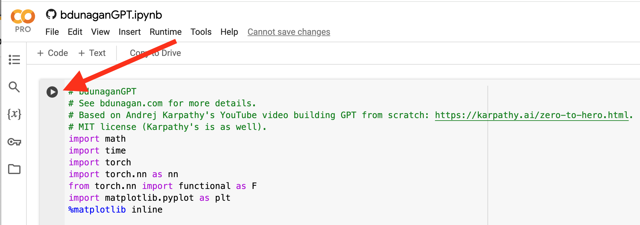
Google Colab will run this notebook: training the 10-million parameter model, running inference, and outputting 100 new tokens––in 10 minutes for free using the T4 GPU with the following hyperparameters:
GPTTest(batch_size=32, block_size=128, max_iters=1400, learning_rate=1e-3, n_embd=128, n_head=4, n_layer=52, dropout=0.1, device=device)
The model achieves a loss of 1.680 and produces the following text:
"Store 200 nice detail handled details of Launch and files or an useful base Amazon Vier. I also read"
Some people will find this output astonishing. Others will find it laughably bad. Both are right. The difference is in expectation and understanding of the building blocks of the neural network.
Before training, the model knows nothing; it doesn’t understand or write English. Its only training for knowing what character (token) to write next is based solely on my blog’s contents. After running a training loop one thousand times on one GPU, the model was able to string together characters into English words, capitalize the first word, and add some spaces and even a period. It’s not ChatGPT though, which took months to train on thousands of GPUs with billions of tokens.
This model is based on Andrej Karpathy’s excellent nanoGPT model from his Zero-to-Hero YouTube course, a fantastic and accessible deep dive into deep neural networks. Karpathy is a cofounder of OpenAI and was the Director of AI at Tesla before recently returning to OpenAI. Learn about how to write a model like this in his “Let’s build GPT: from scratch, in code, spelled out” YouTube video.
I updated the Python code in three ways:
- Pytorch’s Multihead Attention: I switched from Karpathy’s version of Multihead Attention to Pytorch’s version using an attention mask.
- Positional Encoding: I experimented with the original
sin()andcos()positional encoding function with no learning parameters from Google’s “Attention Is All You Need” paper, but testing showed that Karpathy’s simpler learned positional encoding reduced loss a bit more. - Toggles: I added three different toggles to experiment with changing the model architecture. Two of them were the above items, and the third was disabling residual connections.
None of my changes improved the model’s original performance, but they were useful for experimentation.
Let’s compare it to GPT-3, using the table from OpenAI’s 2020 research paper titled “Language Models are Few-Shot Learners”:
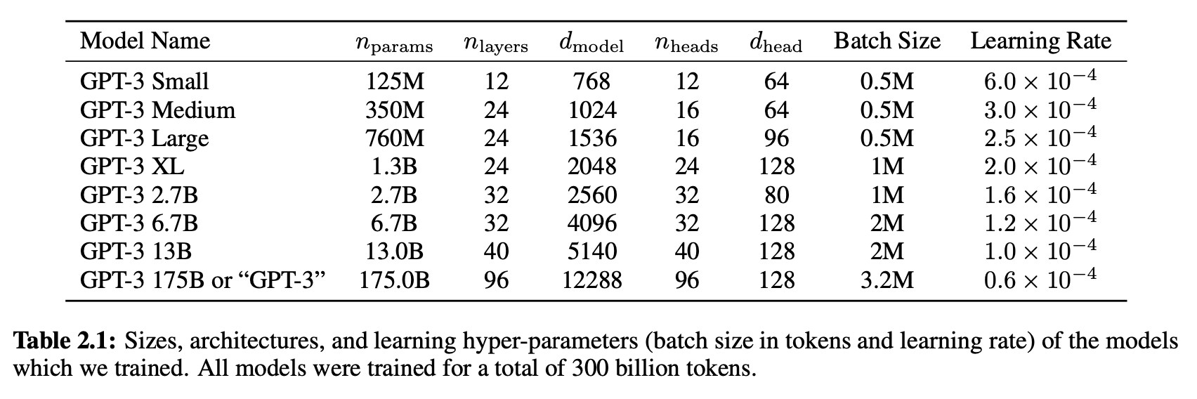
Hyperparameters are attributes about the model and training, rather than weights within the model that we’re tuning. Each of these models was trained on 300 billion tokens, meaning each model had the same massive set of training data to learn from, but there are a number of hyperparameters listed that define the structure of each model. Let’s walk through each hyperparameter, including the equivalent variable name in our bdunaganGPT version:
- nparams (
parameters): The number of total weights (parameters) in the model. - nlayers (
n_layer): The number of aggregate layers in the model. Each layer is composed of multiple components. - dmodel (
n_embd): The dimensionality of the embedding vector. - nheads (
n_head): The number of attention heads in each multi-head attention block. - dhead (
head_size): The number of inputs on each attention head block, determined by two above hyperparameters:n_embd // n_head. - Batch Size (
batch_size): The number of examples in each batch as it’s processed. - Learning Rate (
learning_rate): The step size of how much we update the weights on every back propagation. - Context Window (
block_size): The number of tokens each model reads in to predict the next token. All GPT-3 models used 2048 tokens.
With these hyperparameters, OpenAI configured GPT-3, just like we configured bdunaganGPT. GPT-3 is the same basic architecture as the model we ran. GPT-3 is just much bigger.
There is a significant caveat that models on the scale of GPT-3 can be optimized in various ways. For instance, OpenAI’s paper on GPT-3 refers to “alternating dense and locally banded sparse attention patterns in the layers of the transformer, similar to the Sparse Transformer.” But broadly speaking, the architectures are the same.
Training
The loss calculation is independent of our architecture, so we can test the loss with different architectures, processors, and hyperparameters to see which minimizes the training times and loss. For instance, doubling the layers might reduce the loss by a bit but double the training time, which might be an unacceptable tradeoff. I used cross entropy loss as the loss function for the model feedback. It’s the same as negative log likelihood and is derived from KL divergence.
Let’s look at how the loss decreases over time. With random weights, the loss should be around -ln(1/n) where n is the number of possible tokens. In my case, there are 107 possible characters in bdunagan.com.txt, so the baseline loss is around 4.8. The loss quickly decreases though. By saving the loss for each iteration, we use Matlab to plot how the loss changes over time.

plt.plot(steps, losses)
The significant noise in the loss graph is caused by the variance in the batches. As the LLM progressively trains across different batches, the loss goes up and down locally while still decreasing on average, and the plot visually confirms that the model is improving with more training.
The problem is that this model is just one combination of hyperparameters. There could be a different set that produces an even better model. In theory, we could test each combination of hyperparameters to find the optimal one, but in practice, large models take months to train. We cannot exhaustively search the possible space for the minimum loss.
To get a sense of how the loss changes, let’s look at a small set of combinations, all tested on Google Colab’s T4 processor:
| Hyperparameters | #1 | #2 | #3 | #4 |
|---|---|---|---|---|
| Parameters | 5,451 | 31,339 | 212,331 | 1,621,611 |
| Layers | 4 | 8 | 16 | 32 |
| Embedding Vector | 8 | 16 | 32 | 64 |
| Heads | 4 | 8 | 16 | 32 |
| Batch Size | 8 | 16 | 32 | 64 |
| Block Size | 32 | 128 | 128 | 256 |
| Learning Rate | 1e-2 | 1e-3 | 1e-4 | 1e-5 |
| Dropout | 0.0 | 0.1 | 0.2 | 0.3 |
| Iterations | 1,000 | 1,000 | 1,000 | 1,000 |
| Training Time(s) | 19 | 36 | 77 | 1218 |
| Validation Loss | 2.627 | 2.588 | 2.770 | 3.253 |
More parameters doesn’t immediately translate to lower loss. By decreasing the learning rate for the 1.6m-parameter model, we saw a higher loss than the 30k-parameter model after the same number of training iterations.
Even with one particular hyperparameter combination, more training isn’t always better. As an example of overfitting, see the table below to watch the validation loss grow while the training loss continues to shrink. The set of parameters shows that even the number of iterations is important.
| Iterations | Training Loss | Validation Loss |
|---|---|---|
| 500 | 2.0993 | 2.1271 |
| 1,500 | 1.2805 | 1.6006 |
| 3,000 | 0.9815 | 1.7457 |
Unsurprisingly, changes to the Transformer architecture lead to significant changes in the final loss. Let’s see the effect of disabling various parts of a 200k-parameter model over 2,000 iterations with the following hyperparameters: 4 layers, 4 heads, 16 batch size, 32 block size, 1e-3 learning rate, 64 embedding vector, and 0.0 dropout.
| Model Notes | Validation Loss |
|---|---|
| Original architecture | 1.916 |
| No normalization | 1.926 |
| No positional encoding | 2.026 |
| No attention | 2.554 |
| No residual connections | 3.162 |
At this small scale, certain architectural pieces are less necessary than others are. Attention is the fundamental insight of the “Attention Is All You Need” paper from Google, and that layer is clearly helpful at capturing information for the model to use.
However, the effect of residual connections is even more powerful. These connections are the + operations that add the input to the output of a layer, and backprogagation over residual connections lets the model avoid vanishing gradients because the final loss flows back to each layer separately, thanks to the derivatives. (Watch Karpathy’s micrograd YouTube video for a detailed mathematical explanation.) By cobbling together these architectural patterns, we can avoid plateauing in the loss function over many training iterations.
All these training passes take time, but the processor type drastically changes how long. Let’s compare how long training takes for different processors that Google Colab has available.

We’ll use the 800k-parameter LLM to accentuate the differences in times with the following hyperparameters: 16 layers, 1,000 iterations, 8 heads, 64 batch size, 128 block size, 1e-3 learning rate, 64 embedding, and 0.0 dropout. Note that Google Colab provides CPU and T4 for free when resources are available, but the A100 and V100 are part of the paid plan.
| Processor | Training Time (seconds) |
|---|---|
| CPU | 7568 |
| T4 GPU | 117 |
| V100 GPU | 69 |
| A100 GPU | 64 |
GPUs greatly accelerate training performance, even in this very small example. The model trained in two hours on the CPU and in one minute on the GPU. The Nvidia A100 GPU enabled the model to train 118x faster than the CPU did, opening up opportunities for scaling that wouldn’t have been practical with CPUs.
Inference
We’ve quantified the loss across a variety of different hyperparameters, but we have no idea what the output looks like for each tier of loss. Again, before training, the model knows nothing about English. During training, all it sees is my blog’s content and tries to replicate it to mimimize the loss. Let’s qualify the loss by see the output text at various points:
4.0 Validation Loss:
==rv8\
Exlu(6~@ '/)1/U⌘N4vbyYW&?jeuP48-ea>"6\\R
;J!>:3~ "H~25 V" djP1Qw%uI<\d”>—y7 dna+ZHa%Cal<(-:?7
3.0 Validation Loss:
T .septheeh.s 9 nt> e yr. ye dmnild
a .aueo_r%lme ol e aslen r hu.noco W Un elenQdhautf t neep
2.5 Validation Loss:
alder t Cfo t o s TalySL mlo deo dotersincolrwfit rto me ontade. iom Pk gs "indodeacronero andn. t'
2.0 Validation Loss:
ayigh, Ontiss thippated to so peckup to with spoickin't nox a rele davestrn difUpearanges and frotuI
1.6 Validation Loss:
I going turn into a key-vs, partners, remarker of these; additions tha steps disconsforw was easy li
Look at how the text changes from random letters to almost coherent words and then to almost reasonable sentences. A magical quality of deep neural networks and LLMs in particular is the ability to continually decrease the loss with the right hyperparameters and more data in a reasonable amount of time with GPUs. They continue to absorb more context and leverage that knowledge to generate new tokens that accurately resemble the existing data set.
Fine-Tuning
What we built is not ChatGPT. What we did is referred to as pre-training. The model is trained on a large corpus with a loss function that measures how well the output matches the corpus. Regardless of how much we improved the loss, the output would remain a steady stream of sentences that sound like my blog posts, not answers to questions.
The next step is called fine-tuning, feeding in thousands of examples of conversations along with reinforcement learning with human feedback (from) to nudge the models’ pre-trained weights to appear to respond to questions with answers or write accurate responses to prompts.
Leaky Abstraction
There is a significant difference between reading about machine learning and large language models and actually attempting to create one. At one point during his YouTube series, Karpathy notes that deep neural networks are a “leaky abstraction”: understanding the internals of each aspect is critical to avoid pitfalls. Let’s look at three different instances in our simple model:
- Hyperparameter Tuning: Simply increasing the iterations for certain hyperparameter combinations increased our model’s validation loss rather than decreasing it. Overfitting is a huge problem in machine learning in general.
- Residual Connections: Before these connections, models suffered from vanishing gradients because the loss function’s output didn’t flow back to each layer separately and instead passed through each layer. But without understanding the math behind how the derivative can bypass layers with an addition, it wouldn’t be clear that residual connections would be a way around that. See the following code blocks as a comparison:
# Residual connection in Transformer Block
x = x + self.sa(self.ln1(x))
x = x + self.ffwd(self.ln2(x))
# No residual connection in Transformer Block
x = self.sa(self.ln1(x))
x = self.ffwd(self.ln2(x))
# Subtle bug in residual connection in Transformer Block
x = self.ln1(x) # BUG: x is overridden and no longer passes through, but this works for small networks
attn_mask = nn.Transformer.generate_square_subsequent_mask(T).to(self.device)
output, _ = self.sa(x, x, x, attn_mask=attn_mask, need_weights=False, is_causal=True)
x = x + output
x = x + self.ffwd(self.ln2(x))- Matrix, Layer, and Model Analysis: Every level of the model requires analysis and optimization to reduce the loss to the minimum, including studying matrix sizes to ensure they are doing what they are expected to do and making sure the network is set up correctly. These systems are incredibly complex at scale, with a host of places that could silently increase loss.
Understanding the innerworkings of neural networks enables us to optimize and tune models in a way that relying on the abstraction would not.
Moreover, a deeper knowledge both demystifies and highlights the magical quality of LLMs. ChatGPT is an LLM that frequently feels like talking to a person. Fundamentally, it is an LLM that is simply predicting the most appropriate next token in a way that minimizes the loss. I still find it amazing that these steps can lead to such an authentic interaction.