March 16 2024

A Glossary for Understanding Large Language Models in AI such as OpenAI's GPT-4, Meta's Llama2, and Google's Gemini

by Brian Dunagan

OpenAI’s GPT-4, Meta’s Llama2, and Google’s Gemini are all forms of large language models (LLMs), a subset of deep neural networks, which are a subset of machine learning algorithms. LLMs feel magical, but at their core, these models are token-prediction algorithms. The fundamental building blocks of these machine learning models are quite simple but capable of achieving astounding results at scale.

Let’s walk through a number of words that come up for LLMs.

Glossary

At the highest level, we care about two aspects:

• Model: The model is the actual algorithm for processing a given input context and generating an output.

• Weights: Weights are numerical constants being multiplied with (weights) or added to (biases) the inputs, like (w*x + b). For simplicity, weights and biases are both referred to as weights. They’re also referred to as parameters. GPT-3 has 7 billion parameters. Talking about the number of weights for a neural network gives an instant scope to the complexity of the network, but the number does not translate into accuracy.

Going a level deeper, we can think about how we train and use the model and weights:

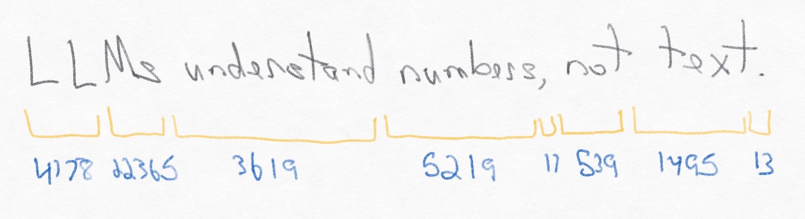
• Tokens: GPT-3 was trained on a massive corpus of text. However, neural networks don’t “read” text. They take a set of numbers as input and output a set of numbers that minimize the loss function. These numbers are called tokens. For large language models (LLMs), text is converted into these tokens that typically represent subword chunks (not individual characters but not words) for the network to read as input and to write as output.

• Training: To optimize the weights of the neural network, we take a large corpus of data and iteratively run a forward pass (inference) on small sections of it to generate an output. The output is then compared to our desired output, and the difference is called the loss. The loss is passed backwards through the network using calculus to adjust the weights, so that the next forward pass is more accurate. The goal of training is to minimize the loss of a model’s inference.

• Inference: When consumers use ChatGPT, the model is running inference (a forward pass) to read an input to generate an output.

Below models and weights, we can dive into the innerworkings of neural networks. Let’s go through them in quasi-top-down order:

• Hyperparameters: These refer to the actual configuration of the neural network, like having 2 layers of 100 neurons or 4 layers of 50 neurons. Optimizing hyperparameters is a second-order optimization on top of optimizing the weights of one iteration of the neural network.

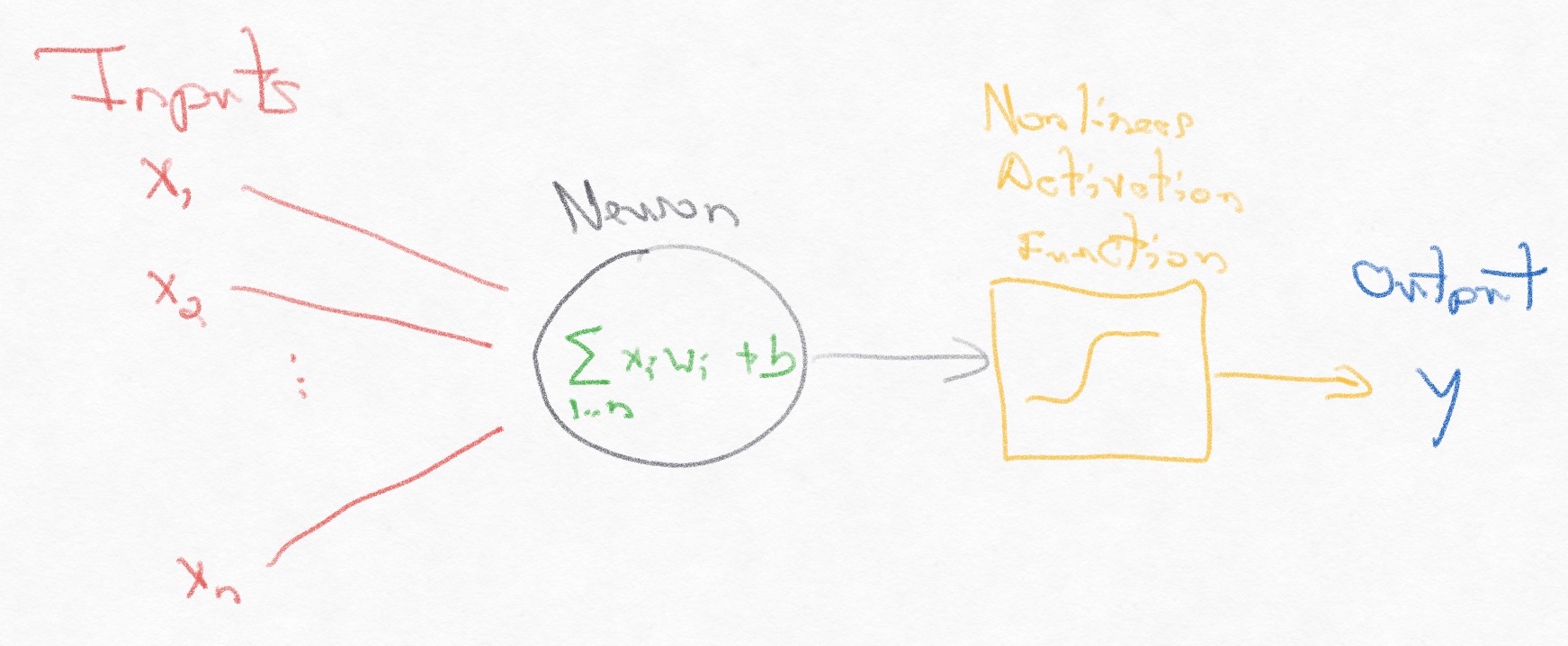
• Neuron: The neuron, also referred to as a node or a perceptron, is the central building block of the neural network. It’s a simple mathematical function, designed to represent a biological neuron. The neuron takes a set of input values (x_n), multiplies each by a weight (w_n), adds them all together, adds a bias (b), and finally passes that value through a non-linear function, also called an activation function, to produce an output (y).

• Loss Function: The loss function is the final part of the neural network, only present during training, and compares the output of the forward pass of the network to the expected output. Again, the goal is of training is to minimize the loss.

• Forward Pass: The forward pass of a network is processing an input through the network into an output. For an LLM, the output is a set of probabilities returned by the softmax function to decide the likelihood of the next token within the token space. That probability distribution is then sampled to decide on the predicted token.

• Backward Pass: The backward pass of a network is the crucial part of training neural networks. We take the output of the loss function and feed it into the network going backwards using calculus to take local derivatives of each part with respect to the final output.

• Gradient Descent: When we calculate the derivative of the local equation with respect to the final output during the backward pass, we use the local slope and multiply it by a small learning rate to move toward the local minima.

• Learning Rate: We are using gradient descent to move the weights incrementally toward an output that is the local minima of the equation. The learning rate is the step size of these increments: too small will take the network too long to reach the local minima, too large will cause the network to overshoot the local minima.

• Cross Entropy Loss: We need a loss function to help the neural network learn how to improve based on a single positive number that we want to minimize, and popular ones include cross entropy loss and mean square error (MSE) loss. Cross entropy loss takes the softmax of the logits and then the mean of the negative log likelihood, giving us a single number. Negative log likelihood (NLL) is simply the negative log of the value. The cross entropy loss function is calculating the distance (KL divergence) between the predicted probability distribution and the true probability distribution. Simplifying that mathematical formula results in the negative log likelihood.

• Softmax: This is a normalization function that translates a set of numbers to a set of probabilities between zero and one, enabling the result to be handled as a standard probability range. However, instead of a basic normalization function that divides each value by the sum of all values, softmax uses e^x / sum(e^x). The exponential component both highlights the maximum value by increasing the distance between it and the other values, unlike basic normalization, and is differentiable, unlike hardmax.

• Logits: It’s the unit of measurement for a log scale (logistic unit). We use this term for the output of the penultimate neural network layer before we normalize the output using the softmax function (to get final probabilities for the next token) or before we calculate cross entropy loss (to get a loss number to minimize). Logits are unnormalized log-probabilities because both of those subsequent functions includes a softmax calculation, which exponentiates and normalizes the values. Logits are not the final values because we want the neural network’s output to be in the form of probabilities with the maximum value exaggerated through the softmax function.

• Logprobs: After we use softmax on the output to get the probabilities of the next token, we take the log to get logprobs, and this extra calculation helps with numerical stability for small probability values due to the way computers store real numbers. For example, .000000001 and .0000000001 are 10x different, but their precision could be lost; however, log(.0001) is -9 and log(.00001) is -10, and their precision won’t be lost in storage. Surfacing logprobs from an LLM provides more nuance to the LLM’s confidence in its own output and what alternative responses would have been. OpenAI started providing logprobs for its selected output tokens and alternative tokens in 2023.

• Batch Size: The model cannot process the entire training data set in one pass, and it would lose valuable information if it processed each example independently. The batch size refers to the numbers of examples that are processed concurrently in a single forward pass. For example, GPT-3 had a batch size of 3.2 million, so every forward pass had 3.2 million examples to process together to form a better understanding.

• Attention: Neural networks do not automatically absorb relationship information. For example, in the sentence “The house is on the market.”, “house” and “market” have a relationship, but it’s not the same relationship as the two words in the sentence “The house is next to the market.” Previous architectures, like recurrent neural networks (RNNs), add dependencies between stages of the model to add better relationship information, but this dependency prevented them from being efficiently parallelizable. In a 2017 research paper from Google titled “Attention Is All You Need”, researchers proposed capturing that contextual information in a new set of weights to train in the network in the form of matrices called “Query”, “Key”, and “Values”. The paper was focused on machine translation, using an encoder block for the source text and a decoder block for the destination text. However, attention has become the central architectural insight for modern LLMs because models can absorb relationship information of surrounding tokens in an efficiently parallelizable way.

• Cross-Attention: This version of attention has the keys and values come from the encoder while the queries come from the decoder. Cross-attention is tailored to machine translation, where the model is attempting to both understand the source language in its entirety but also understand and predict the destination language output. For example, a model translating French to English would see “Bonne après-midi.” as input to the encoder block but only “Good” (not “ morning”) as input to the decoder block. Its job is to use the entire French context and a partial English context to predict the next English token. Again, this approach has proven in practice to be far better than any other ML algorithm has been.

• Self-Attention: This version of attention has the keys and values generated from the same input as the queries, using a decoder block and no encoder block. Reusing our example, the input would be “Good” as tokens, and based on training data, the model would predict “ afternoon” as the next token.

• Multi-Head Attention: One layer of self-attention only lets us represent a single relationship between two tokens, because the softmax function highlights only one possibility. Adding more heads enables the layer to capture more relationships to absorb more information about the tokens. For example, “The hungry dog ate breakfast.” has multiple relationships: “hungry” and “dog”, “dog” and “ate”, “hungry” and “ate”, “ate” and breakfast”, and “hungry” and “breakfast”. We want the LLM to absorb as many relationships as possible to most accurately predict what to say next.

• Encoder: There can be two modules for attention: an encoder and a decoder. A model for machine translation uses both. The encoder takes the source language, and the decoder takes the destination language. And keep in mind that encoding is not the same as embedding. Moreover, there are decoder-only models like BERT.

• Decoder: The decoder can take a destination language for machine translation, or it can be used outside of machine translation for token prediction, like for GPT.

• Tokenization: The input needs to be translated into numerical values (tokens) for the model to interpret mathematically. This process is called embedding. A single token is pre-assigned a number, so the set of tokens in the input becomes a vector of numbers. The token-to-integer lookup is defined statically in advance. For example, Google uses a sub-word embedding algorithm called sentencepiece, and OpenAI uses one called tiktoken (with 50,257 possibilities).

• Embedding: Tokens are used as a lookup into an N-dimensional vector space, called an embedding space. Each token’s vector is random initially and adjusted through back propagation during training to bring similar tokens closer to each other and dissimilar tokens further from each other. Keep in mind that embedding is not the same as attention and does not retain token positions.

• Positional Encoding: Attention captures relationships between tokens, but it does not include actual position. Encoding the position of each token provides more information for the model to utilize. The 2017 “Attention is All You Need” paper from Google decided to use a sin/cos formula based on the embedding vector dimension, embedding vector index, and token index in order. These encoding values are simply added to the embedding vectors’ values (keeping the dimensionality the same). An alternative approach is to create a second embedding with the dimensions of the context length and the original embedding vector and add that to the original embedding vector. This second option is called learned positional encoding because it lets the neural network optimize the weights and can lead to even better performance.

• Vanishing Gradient: A key insight in the attention paper was adding the raw input of a layer to the layer’s output through a residual connection. The backpropagation calculus lets the gradient pass back to the initial layers without being diminished by intermediate layers, improving the learning rate. Other architectures found the gradient vanished as it traveled back through the layers.

• Context Window: As token-prediction algorithms, LLMs take an input to produce exactly one token. The first inference produces the first output token, based on the input. The second inference produces the second token, based on the input and the first output token. And the process continues, sliding the context window along by one token per inference run. When using ChatGPT, the displayed response is actually the model being run over and over again to take the question and on-going response to produce the next token.

• Context Length: This is the total number of tokens that the neural network can take as input. In papers, researchers refer to this as the block size. Because it’s the total, LLMs like GPT include the output token length in the count, so that the LLM can keep the beginning of the input in the context window while generating the end of the output. Otherwise, the LLM would “forget” what the beginning of the initial input was while attempting to generate the end of the output.

• Labeled Data Set: Training a model requires an input and a desired output, referred to as the label. The model trains its parameters to minimize the difference (loss) between the actual output and the desired output. For the text prediction tasks that an LLM performs, the label is the next token in the data set. This data set is split into three subsets: training data set (60%), validation data set (20%), and test data set (20%). (Percentages vary.) Consumer LLMs like ChatGPT are trained on huge data sets. For instance, GPT-3 was trained on 300 billion tokens, so in our breakdown, that would be 180 billion tokens for the training set, 60 billion tokens for the validation set, and 60 billion tokens for the test set.

• Training Data Set: This subset of data is used to actually train the model.

• Validation Data Set: This subset of data is used to validate the loss of the model but not training the model, such as running many different configurations of hyperparameters and finding the lowest loss. At a higher level though, the model is being trained on this subset simply by optimizing for the model where those hyperparameters generate the lowest loss.

• Test Data Set: This subset of data is used to test the loss of the final model using data that the model has never seen to identify underfitting or overfitting.

• Overfitting: By training models on a specific set of data, the parameters can become too optimized on its quirks. For instance, training a model on thousands of pictures of a cow in a grass field might lead to a model that cannot identify a cow standing on a road. It extracted the wrong information from the data and overfit: no grass, no cow.

• Underfitting: If the model does not have access to enough data, it can underfit and not be able to complete the task. In the example of the cow in a grass field above, training a model on only ten images of cows would not provide enough information for the model to be able to identify a cow in a new image. Well-tuned models neither overfit nor underfit; they absorb enough information to complete the task but are able to generalize beyond the trained data set to work on new inputs.

• Zero-Shot Learning: A model is able to complete a task without ever having seen it before. ChatGPT was so surprising because it did very well at tasks that it had never been trained on, like “write a haiku about why ChatGPT’s service is overloaded” (which OpenAI had on its status page for a while).

• Few-Shot Learning: A model is able to complete a task having only seen a couple instances of it before.

• PyTorch: This is a popular Python library created by Meta (then Facebook) for writing machine learning. It’s a complement to Pandas and numpy libraries and competes with Google’s Tensorflow.

• Pre-training: “Training” encompasses the entire process of preparing a model for usage, but technically, optimizing weights is referred to as pre-training.

• Fine-Tuning: After pre-training a model, we use a smaller set of examples, on the order of thousands, to fine-tune the weights of the model to solve more specific tasks, such as answering questions.

Finally, let’s touch on a number of general terms that come up for the current state of machine learning:

• Transformers: This is a type of neural network architecture that Google researchers proposed in 2017 in “Attention Is All You Need” that utilizes attention as a building block. It’s called a transformer because the model transforms the data in different ways and the model needed a name to differentiate itself from RNNs, which were the state-of-the-art at the time.

• GPT: This is an acronym for generative pre-trained transformers that OpenAI came up with, first seen with their GPT-1 model. ChatGPT has been so successful that transformer and GPT are frequently used interchangeably.

• LLM: This is an acronym for large language models. GPT is a specific type of LLM.

• Foundational Model (FM): This is a type of AI model that has been trained on a large set of data and can be applied to a large set of use cases. Due to the success of ChatGPT and other LLMs, there is a growing set of companies operationalizing foundation model pipelines, referred to as FMOps or LLMOps.

• Multi-Layer Perceptron: This is a simple type of neural network that has multiple layers of perceptrons, also referred to as neurons.

• Convolutional Neural Networks (CNNs): Commonly used for image analysis, this type of neural network has convolutional layers in between feedforward (unidirectional) layers. These convolutional layers act as filters on the data, sliding across the context and extracting certain features into its weights. Google DeepMind released a popular version called WaveNet for processing audio.

• Recurrent Neural Networks (RNNs): Before transformers, this was the best neural network for machine translation. It preserves state inside each layer to use the previous output in the next input, giving the network a memory but also introducing dependencies between iterations and neurons. For comparison, the attention architecture in transformers also adds a form of memory but without the dependencies, so transformers can parallelize more efficiently.

• Small Language Models (SLMs): Given the success of ChatGPT, companies are exploring how to build their own small-scale models but with a small set of domain-specific data to focus the model on a set of tasks. General LLMs like GPT-4 and Gemini take months to train and significant resources even for inference. Shrinking the number of parameters makes the model smaller and more efficient without reducing performance at specific tasks, to the point where these models can run on-device instead of in a data center via the cloud.

Foundation

Neural networks have been around for decades, but access to data and compute power at scale has enabled these models to cross a threshold from useful to magical. ChatGPT became an instant sensation because people did not realize a computer could respond to questions like a person. Still, at its core, a large language model such as ChatGPT is a token-prediction algorithm, and understanding how an LLM is built helps demystify and ground its performance. This glossary provides a reasonable foundation for understanding the details.